Abstract
Autoencoders represent an effective approach for computing the underlying factors characterizing datasets of different types. The latent representation of autoencoders have been studied in the context of enabling interpolation between data points by decoding convex combinations of latent vectors. This interpolation, however, often leads to artifacts or produces unrealistic results during reconstruction.
We argue that these incongruities are due to the structure of the latent space and because such naively interpolated latent vectors deviate from the data manifold.
In this work, we propose a regularization technique that shapes the latent representation to follow a manifold that is consistent with the training images and that drives the manifold to be smooth and locally convex. This regularization not only enables faithful interpolation between data points, as we show herein, but can also be used as a general regularization technique to avoid overfitting or to produce new samples for data augmentation.
Motivation
- Autoencoder latent spaces are non-convex: While they represent an effective approach for exposing latent factors, autoencoders demonstrate visible artifacts while interpolating a convex sum of latent vectors.
- GANs are not bidirectional: To interpolate between two real data points, we must map the datapoints back into latent space where admissible interpolation can be performed. Such inverse mapping is not a part of the GAN framework. Additionally, the latent space of the GAN does not necessarily encode a smooth parameterization of the data.
Manifold Data Interpolation
Before presenting the proposed approach we would like to define what constitutes a proper interpolation between two data points. There are many possible paths between two points on the manifold. Even if we require the interpolations to be on a geodesic path, there might be infinitely many such paths between two points. Therefore, we relax the geodesic requirement and define less restrictive conditions.
Formally, assume we are given a dataset sampled from a target domain \(\cal{X}\). We are interested in interpolating between two data points \( \boldsymbol x_i \) and \( \boldsymbol x_j \) from \(\cal{X}\). Let the interpolated points be \( \hat{\boldsymbol{x}}_{i \rightarrow j}(\alpha) \) for \( \alpha \in [0,1] \) and let \(P(\boldsymbol x)\) be the probability that a data point \(\boldsymbol x\) belongs to \(\cal{X}\).
We define an interpolation to be an admissible interpolation if \( \hat{\boldsymbol{x}}_{i \rightarrow j}(\alpha) \) satisfies the following conditions:
-
Boundary conditions: \( \hat{\boldsymbol{x}}_{i \rightarrow j}(0) = \boldsymbol x_i \) and \( \hat{\boldsymbol{x}}_{i \rightarrow j}(1) = \boldsymbol x_j \)
-
Monotonicity: We require that under some defined distance on the manifold \( d(\boldsymbol x,\boldsymbol x’) \) the interpolated points will depart from \( \boldsymbol x_i \) and approach \( \boldsymbol x_j \), as the parameterization \( \alpha \) goes from \(0\) to \(1\). Namely, \( \forall \alpha’ \geq \alpha \):
\[ d(\hat{\boldsymbol{x}}_{i \rightarrow j}(\alpha), \boldsymbol x_i ) \leq d(\hat{\boldsymbol{x}}_{i \rightarrow j}(\alpha’),\boldsymbol x_i) \]
and similarly:
\[ d( \hat{\boldsymbol{x}}_{i \rightarrow j}(\alpha’), \boldsymbol x_j ) \leq d(\hat{\boldsymbol{x}}_{i \rightarrow j}(\alpha),\boldsymbol x_j) \]
-
Smoothness: The interpolation function is Lipschitz continuous with a constant \(K\):
\[ || \hat{\boldsymbol{x}}_{i \rightarrow j}(\alpha), \hat{\boldsymbol{x}}_{i \rightarrow j}(\alpha+t) || \leq K | t | \]
-
Credability: We require that \( \forall \alpha \in [0,1] \) it is highly probable that interpolated images, \( \hat{\boldsymbol{x}}_{i \rightarrow j}(\alpha) \) belong to \(\cal{X} \). Namely,
\[ P(\hat{\boldsymbol{x}}_{i \rightarrow j}(\alpha)) \geq 1-\beta \mbox{ for some constant \(\beta \geq 0\)} \]
Proposed Approach
Following the above definitions for an admissible interpolation, we propose a new approach, called Autoencoder Adversarial Interpolation (AEAI), which shapes the latent space according to the above requirements.
For pairs of input data points \( \boldsymbol{x}_i, \boldsymbol{x}_j\), we linearly interpolate between them in the latent space: \( \boldsymbol{z}_{i \rightarrow j}(\alpha) = (1-\alpha) \boldsymbol{z}_i + \alpha \boldsymbol{z}_j \), where \( \alpha \in [0,1] \).
-
The first loss term \( {\cal L}_R \) is a standard reconstruction loss and is calculated for the two endpoints \( \boldsymbol{x}_i \) and \( \boldsymbol{x}_j \):
\[ \cal{L}_{R}^{i \rightarrow j} = \cal{L}(\boldsymbol{x}_i,\hat{\boldsymbol{x}}_i) + \cal{L}(\boldsymbol{x}_j,\hat{\boldsymbol{x}}_j) \] where \({\cal L}(\cdot,\cdot)\) is some loss function between the two images.
-
We use a discriminator \( D(\boldsymbol{x})\) to differentiate between real and interpolated data points to encourage the network to fool the discriminator so that interpolated images are indistinguishable from the data in the target domain \(\cal{X}\).
\[ \cal{L}_A^{i \rightarrow j}= \sum_{n=0}^{M} -\log D(\hat{\boldsymbol{x}}_{i \rightarrow j}(n/M)) \]
-
The cycle-consistency loss \(\cal{L}_C\) encourages the encoder and the decoder to produce a bijective mapping: \[ \cal{L}_{C}^{i \rightarrow j}= \sum_{n=0}^{M} | \boldsymbol{z}_{i \rightarrow j}(n/M)- \hat{\boldsymbol{z}}_{i \rightarrow j}(n/M)|^2 \]
where \(\hat{\boldsymbol{z}}_{i \rightarrow j}(\alpha) =f(g(\boldsymbol{z}_{i \rightarrow j}(\alpha))) \).
-
The last term \(\cal{L}_S\) is the smoothness loss encouraging \(\hat{\boldsymbol{x}}(\alpha)\) to produce smoothly varying interpolated points between \( \boldsymbol{x}_i \) and \( \boldsymbol{x}_j\): \[ \cal{L}_{S}^{i \rightarrow j}= \sum_{n=0}^M \left | {\frac{\partial \hat{\boldsymbol{x}}_{i \rightarrow j}(\alpha) }{\partial \alpha}} \right |^2_{\alpha={n}/M} \]
Putting everything together we define the loss \(\cal{L}_{i \rightarrow j}\) between pairs \( \boldsymbol{x}_i \) and \( \boldsymbol{x}_j\) as follows: \[ \cal{L}^{i \rightarrow j} = \cal{L}_R^{i \rightarrow j} + \lambda_A \cal{L}_A^{i \rightarrow j} + \lambda_C \cal{L}_C^{i \rightarrow j} + \lambda_S \cal{L}_S^{i \rightarrow j} \] where \(\cal{L}_R, \cal{L}_A, \cal{L}_C, \cal{L}_S\) are the reconstruction, adversarial, cycle, and smoothness losses, respectively.
Justification for the proposed approach
The following figure illustrates the justification for the four losses. As seen in Plot A, the images \(\boldsymbol{x}_i, \boldsymbol{x}_j\), which lie on the data manifold in the image space (solid black curve), are mapped back to the original images thanks to the reconstruction loss \(\cal{L}_R^{i \rightarrow j}\). This loss promotes the boundary conditions defined above. The reconstruction loss, however, is not enough as it neither directly affects in-between points in the image space nor the interpolated points in the latent space. Introducing the adversarial loss \(\cal{L}_A^{i \rightarrow j}\) prompts the decoder \(g(\boldsymbol{z}_{i \rightarrow j}(\alpha))\) to map interpolated latent vectors back into the image manifold (Plot B). Considering the output of the discriminator \(D(\boldsymbol{x})\) as the probability of image \(\boldsymbol{x}\) to be in the target domain \(\cal{X}\) (namely, to be on the image manifold), the adversarial loss promotes the credibility condition defined above. As indicated in Plot B, the encoder \(f(\boldsymbol{x})\) (red arrows) might, nevertheless, still map in-between images to latent vectors that are distant from the linear line in the latent space. Adding the cycle-consistency loss \(\cal{L}_C^{i \rightarrow j}\) forces the reconstruction of interpolated latent vectors to be mapped back into the original vectors in the latent space (Plot C). The adversarial and cycle-consistency losses encourage bijective mapping (one-to-one and onto) between the input and the latent manifolds, while providing a realistic reconstruction of interpolated latent vectors.
Lastly, the parameterization of the interpolated points, namely, \(\alpha \in [0,1]\), does not necessarily provide smooth interpolation in the image space (Plot C); constant velocity interpolation in the parameter \(\alpha\) may not generate smooth transitions in the image space. The smoothness loss \(\cal{L}_S^{i \rightarrow j}\) resolves this issue as it requires the distance between \(\boldsymbol{x}_i\) and \(\boldsymbol{x}_j\) to be evenly distributed along \(\alpha \in [0,1]\) (due to the \(L_2\) norm). This loss fulfills the smoothness condition defined above (Plot D). If we consider the latent representation as a normed space representing the manifold distance \(d(\boldsymbol{x}_i,\boldsymbol{x}_j) = |\boldsymbol{z}_i - \boldsymbol{z}_j|\), the linear interpolation in the latent space also satisfies the monotonicity condition defined above.
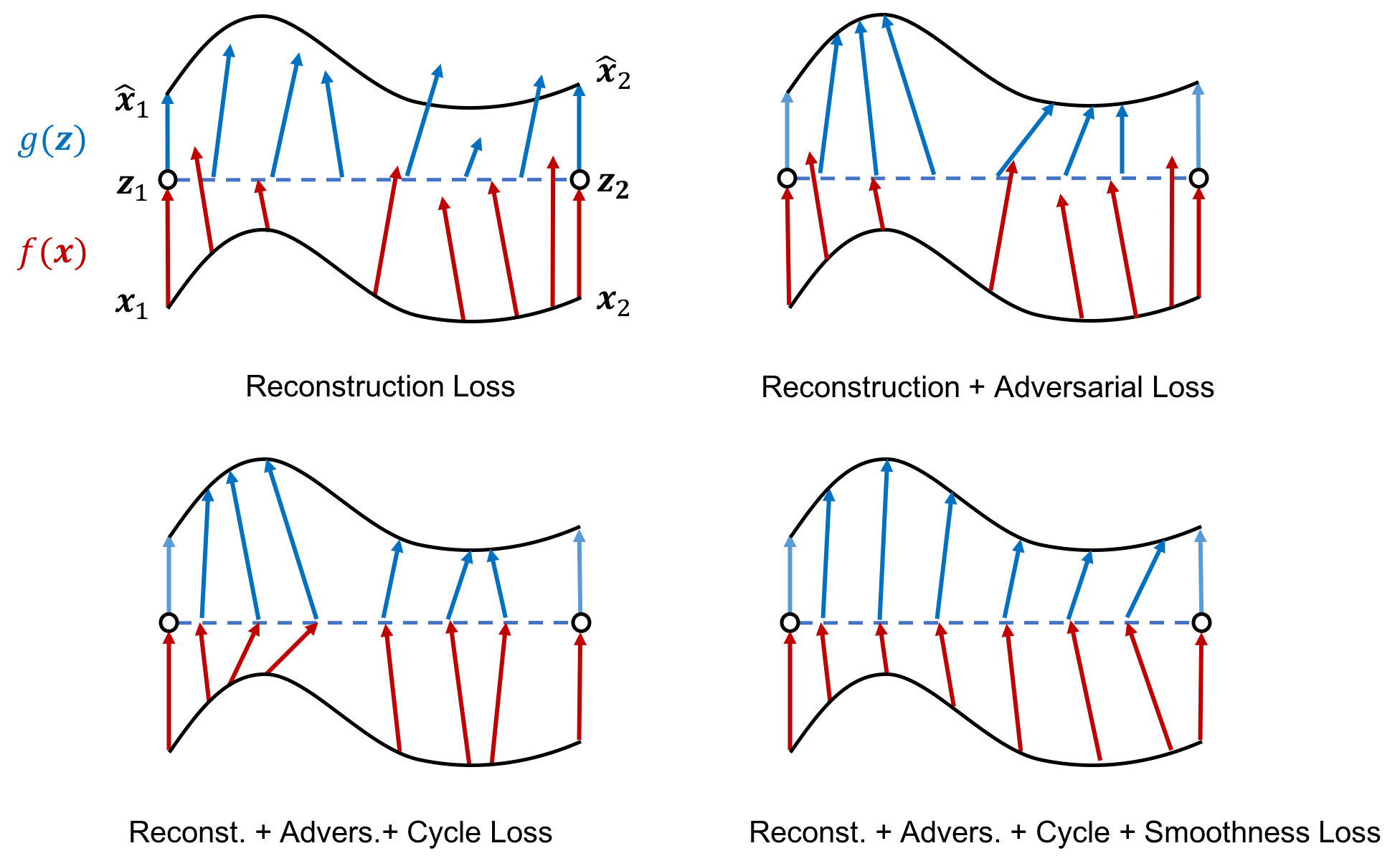
Data interpolation using AEAI. Two points \(\boldsymbol{x}_i, \boldsymbol{x}_j\) are located on the input data manifold (solid black line). The encoder \( f(\boldsymbol{x})\) maps input points into the latent space \(\boldsymbol{z}_i\), \(\boldsymbol{z}_j\) (red arrows). Linear interpolation in the latent space is represented by the blue dashed line. The interpolated latent codes are mapped back into the input space by the decoder \(g(\boldsymbol{z})\) (blue arrows).
Animations
We demonstrate that our technique (AEAI) produces admissible interpolations while other techniques fail to reconsutrct in-between images realistically or to transition smoothly from mode to mode. We tested the following techniques: Adversarial Autoencoder (AAE), Adversarially Constrained Autoencoder Interpolation (ACAI), \(\beta\)-Variational Autoencoder (\(\beta\)-VAE), Generative Adversarial Interpolative Autoencoding (GAIA) and Adversarial Mixup Resynthesis (AMR).
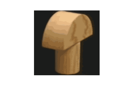
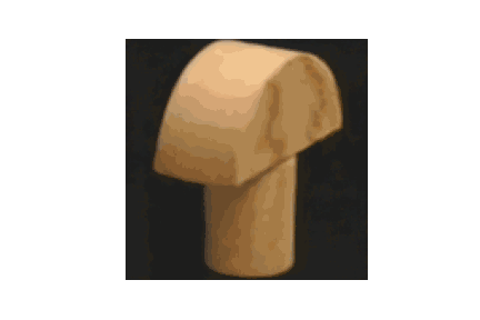
Each animation demonstrates the reconstruction resulting from a linear interpolation in latent space of each method between two images sampled from a testing dataset. The first two animation blocks shows objects from the COIL-100 dataset and the third block shows our synthetic pole dataset.
| AEAI | AAE | ACAI |
|---|---|---|
 |
 |
 |
| \(\beta\)-VAE | GAIA | AMR |
 |
 |
 |
| AEAI | AAE | ACAI |
|---|---|---|
 |
 |
 |
| \(\beta\)-VAE | GAIA | AMR |
 |
 |
 |
| AEAI | AAE | ACAI |
|---|---|---|
 |
 |
 |
| \(\beta\)-VAE | GAIA | AMR |
 |
 |
 |
Results
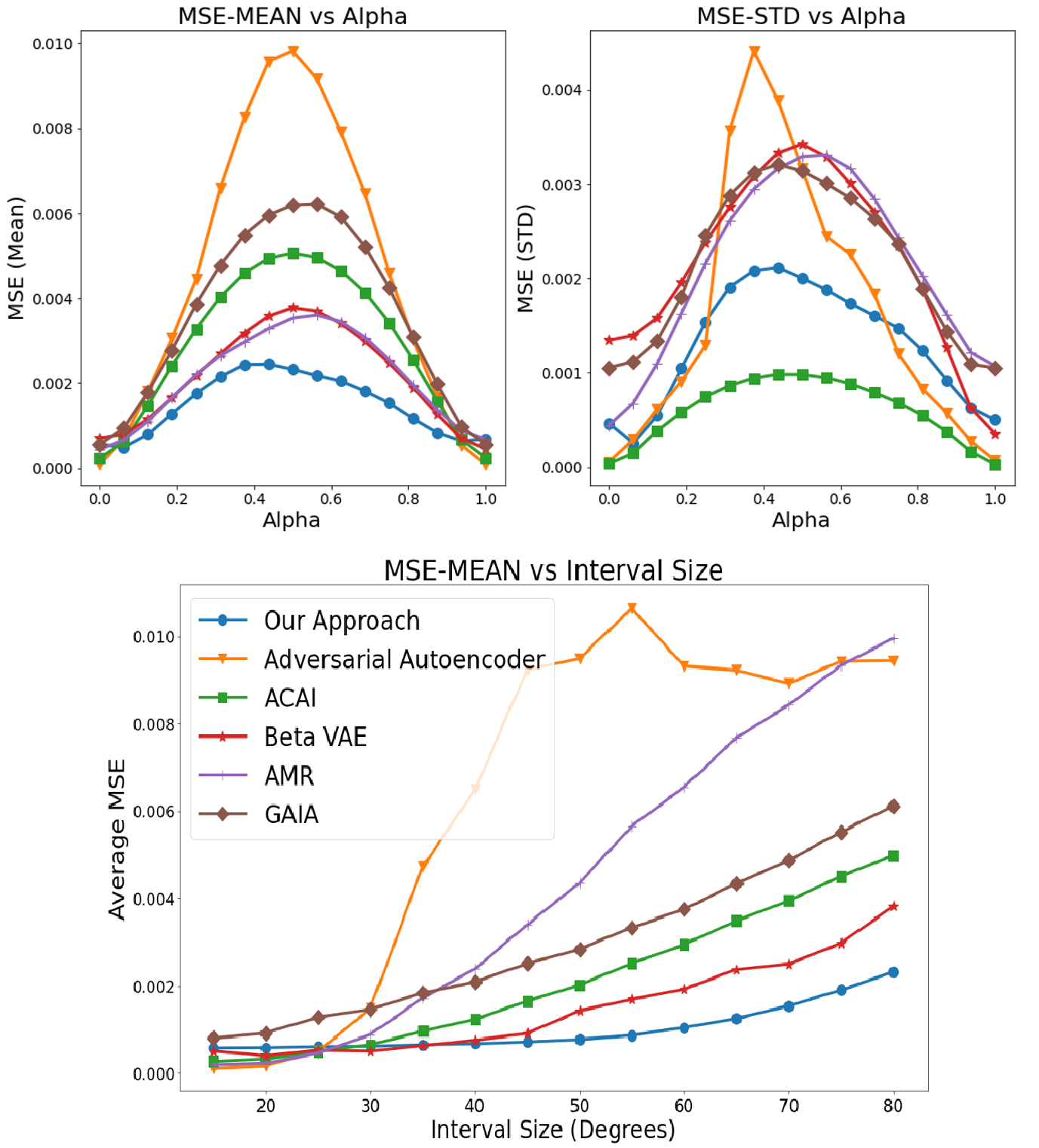
We use the parameterization of the dataset to evaluate the reconstruction accuracy of the AAE, ACAI, \( \beta \)-VAE, AMR, GAIA and our proposed method. Upper left graph: Averaged MSE vs. \(\alpha\) values. Upper right graph: STD of MSE vs. \(\alpha\) values. Lower graph: Averaged MSE of the interpolated images vs. the interval length.
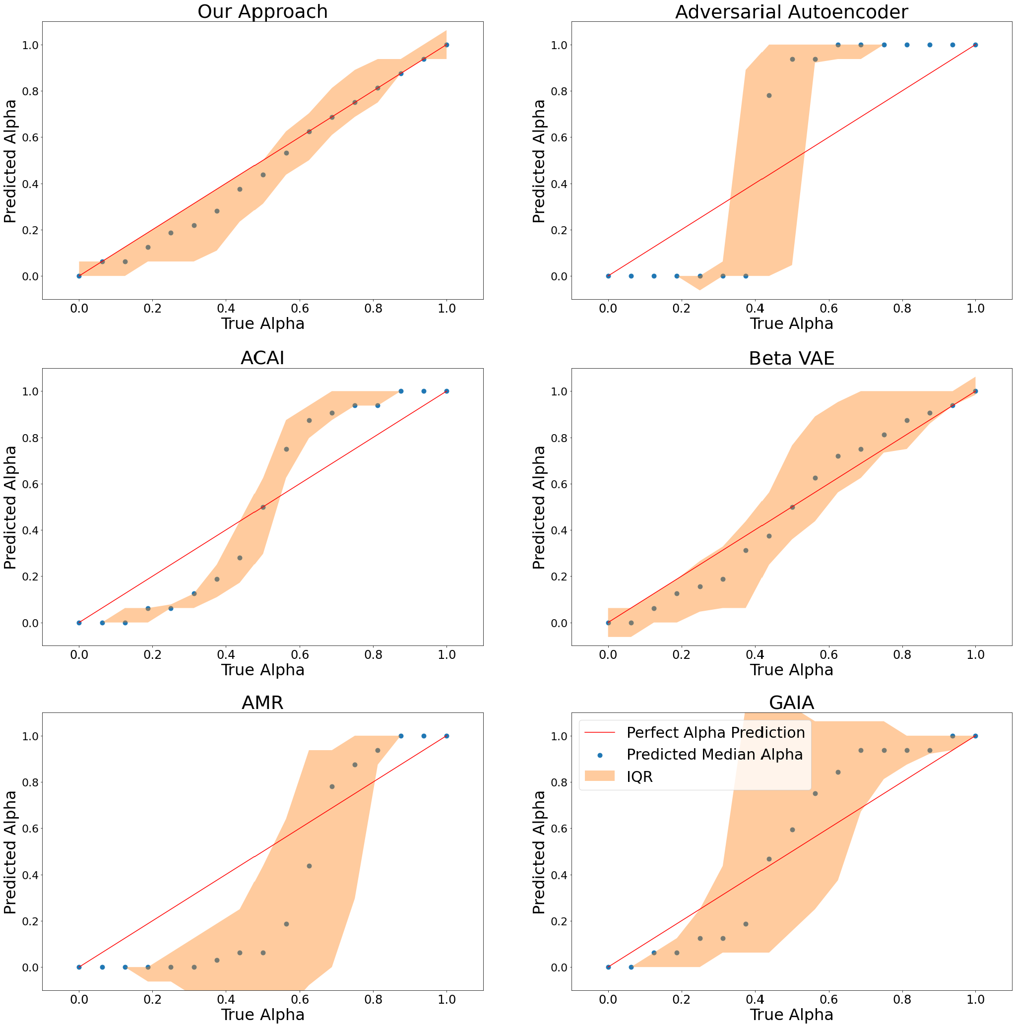
Predicting the interpolated alpha value based on the \(L_2\) distance of the interpolated image to the closest image in the dataset. The dots represent the median and the colored area corresponds to the interquartile range.
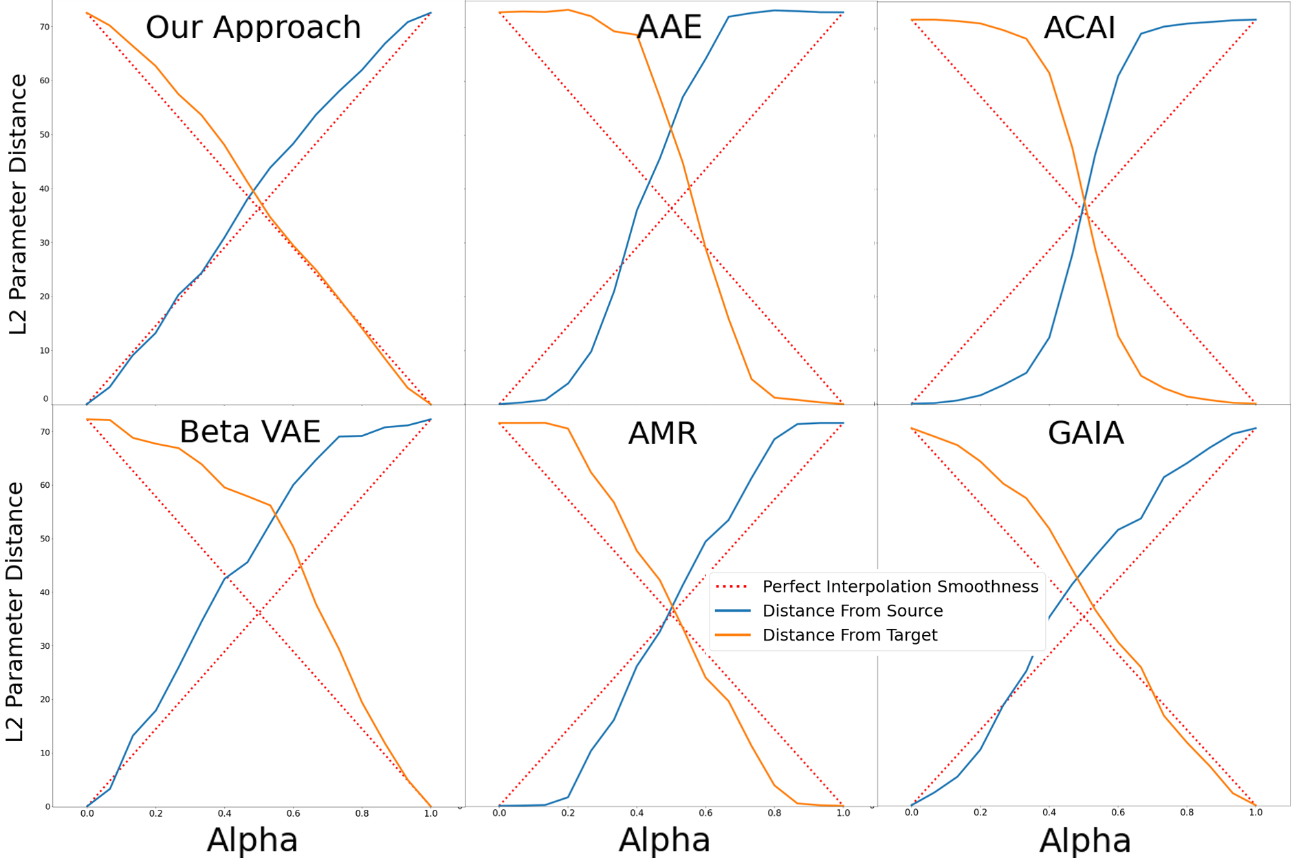
We sampled two images \(\boldsymbol{x}_i, \boldsymbol{x}_j\) and linearly interpolated between them in latent space. For each interpolated image, we retrieved the closest image in terms of MSE from the dataset. The blue and orange lines present the averaged \(L_2\) distance, in the parameter space \((\theta,\phi)\), between the retrieved image and \(\boldsymbol{x}_i, \boldsymbol{x}_j\), respectively. The red lines represent perfect interpolation smoothness.
BibTeX
If you find our work useful, please cite our paper:
@InProceedings{pmlr-v139-oring21a,
  title = 	 {Autoencoder Image Interpolation by Shaping the Latent Space},
  author =       {Oring, Alon and Yakhini, Zohar and Hel-Or, Yacov},
  booktitle = 	 {Proceedings of the 38th International Conference on Machine Learning},
  pages = 	 {8281--8290},
  year = 	 {2021},
  editor = 	 {Meila, Marina and Zhang, Tong},
  volume = 	 {139},
  series = 	 {Proceedings of Machine Learning Research},
  month = 	 {18--24 Jul},
  publisher =    {PMLR},
  pdf = 	 {http://proceedings.mlr.press/v139/oring21a/oring21a.pdf},
  url = 	 {https://proceedings.mlr.press/v139/oring21a.html}
  }